Topic
Retrieving a cell is similar to a spreadsheet vlookup and can save you some keystrokes when setting up tables that use similar data.
Steps
- Build a table with data that you plan to pull into another table. Our table is named Action with columns Name and Activity.

- Build a second table with two columns, Person and Assignment, and name the table Tasks.

- In the Tasks table, select the Person column, and click the Formats button.
Builder tip: The same data is being used in our two tables, but with different names, to make it easier to understand the formulas in later steps.
-
In the Tasks table, format the Person column as Picklist & rowlink that refer to the Action table.
-
Click the chevron in A2 and select a person from the listed choices.

- In B2, type an
=sign, click on the blue name link in A2, click the blue [+] sign to add Action to the formula, and press Enter.

-
Click the chevrons in the Person column to fill out the remainder of the names.
-
Apply the Assignment column formula to the entire column.
a. Click the blue chip in the upper right of cell B2.
This chip notifies you that there is a format mis-match in the column that needs to be addressed.b. Click Apply format to column.
c. Click Apply.

Another way to achieve this
- Switch to Sheets view which allows you to see the entire sheet.

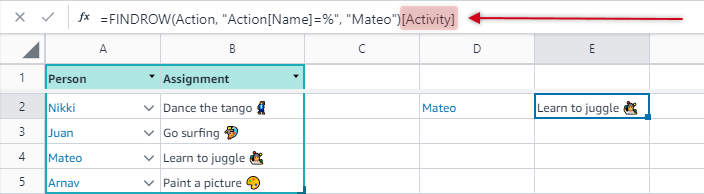
- The FINDROW() function can be used in any cell. Below we are retrieving the cell that includes Mateo from the Action table:
=FINDROW(Action, "Action[Name]=%", "Mateo")

- The same thing goes for retrieving the action. Check out the red highlight in the image to see
[Acticity]being added to the end of the previous step's formula.
=FINDROW(Action, "Action[Name]=%", "Mateo")[Activity]
Going beyond one level
You can go beyond one level so =[Person][Action][Status] is valid if [Action] is a rowlink to a table that contains a [Status] column.

| Was this article helpful? |
|---|
- Yes
- No
0 voters